What are GANs?
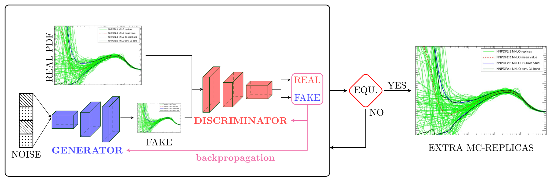
Generative Adversarial Networks are classes of generative-based learning models that given an input data with some probability distribution mathcal{P} generate new data following the same probability distribution by competing two neural network models: a generative model mathcal{G} (Generator) that tries to capture and generate data distribution, and a discriminative model mathcal{D} (Discriminator or Critic) that estimates the probability that a sample came from the input data rather than from the Generator. This adversarial training allows both models to improve over training to the point that the Generator is becoming very good at faking the input data such that the Discriminator can no longer distinguish between generated and input data.
The two neural network models, Generator and Discriminator, are trained together. The Generator generates a batch of samples that along with the samples from the input datad are provided to the Discriminator and classified as real (from the input) or fake (from the generated). The training goes on until equilibrium (Nash Equilibrium) is reached.
Why the need of GANs for PDFs?
Techniques from generative models can be used to improve the efficiency of the PDF compression methodology. IN the standard approach, the task fo the compressor is to extract samples tha present small fluctuations and which reproduce best the statistical properties of the original distribution. It should be therefore possible to use GANs ti generate samples of replucas that contain less fluctuations and once combined with samles from the prior lead t a more efficient compressed representation of the full result.
Discriminator Training
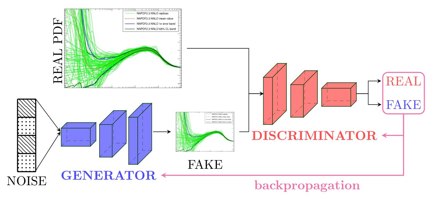
The Discriminator model takes as input MC PDF replicas of shape (NB, NF, X) where NB denotes the number of replica batches, NF the number of flavors, and X the size of the x-grid. The model then outputs predictions as to wether the samples are real with (-1) labels or fake with (1) labels. In different implemtations of GANs, (0) and (1) labels are respectively used to denote the fake and real samples with a Sigmoid as an activation function for the output layer. However, using (-1) and (1) as labels with tanh as activation function is found to be much more efficient. The information as to whether the Discriminator manages to distinguish between real and fake samples is then used to update its weights.
Generator Training
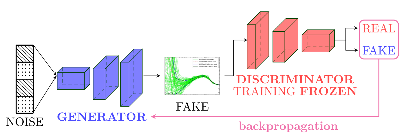
The Generator model takes as input a vector (matrix) of random noise and outputs synthetic MC replicas of shape (NB, NF, X). The Generator’s outputs are then fetch into the Discriminator. During the training of the Generator, it is important that the Discriminator is freezed; otherwise equilibirum might never be reached.
Hyperoptimization
Hyperoptimization or hyper-parameter tuning refers to the automatic optimizations of the hyper-parameters of a Machine Learning model. We refer to hyper-parameters all the parameters of a model that are not updated during the training such as the number of layers, the activation functions, and the algorithm used to minimize the cost function(s). Such optimization (tunning) allows us to search for the best values of hyper-parameters through an hyper-parameter space.
Fréchet Inception Distance (FID)
An important part of the hyper-parameter tuning is the definition of a metric that assesses the goodness of the model. In context of GANs (for PDFs), such a quantity must measure the quality of the generated PDF replicas. To evaluate the performance of the GAN model, we use the Fréchet Inception Distance (FID) [1].
The Fréchet Inception Distance between a multivariate Gaussian with mean \(\mu_{r}\) and covariance \(\Sigma_{r}\) and a multivariate Gaussian wit mean \(\mu_{g}\) and covariance \(\Sigma_{g}\) (where \(r\) and \(g\) resp. denotes samples from real and generated) is given by:
Thus, the lower the value of the FID is, the closer the generated PDFs are to the priors; if the generated PDFs are exactly the same as the input MC PDFreplicas, then the value of the FID is zero.
Optimization Algorithm: TPE
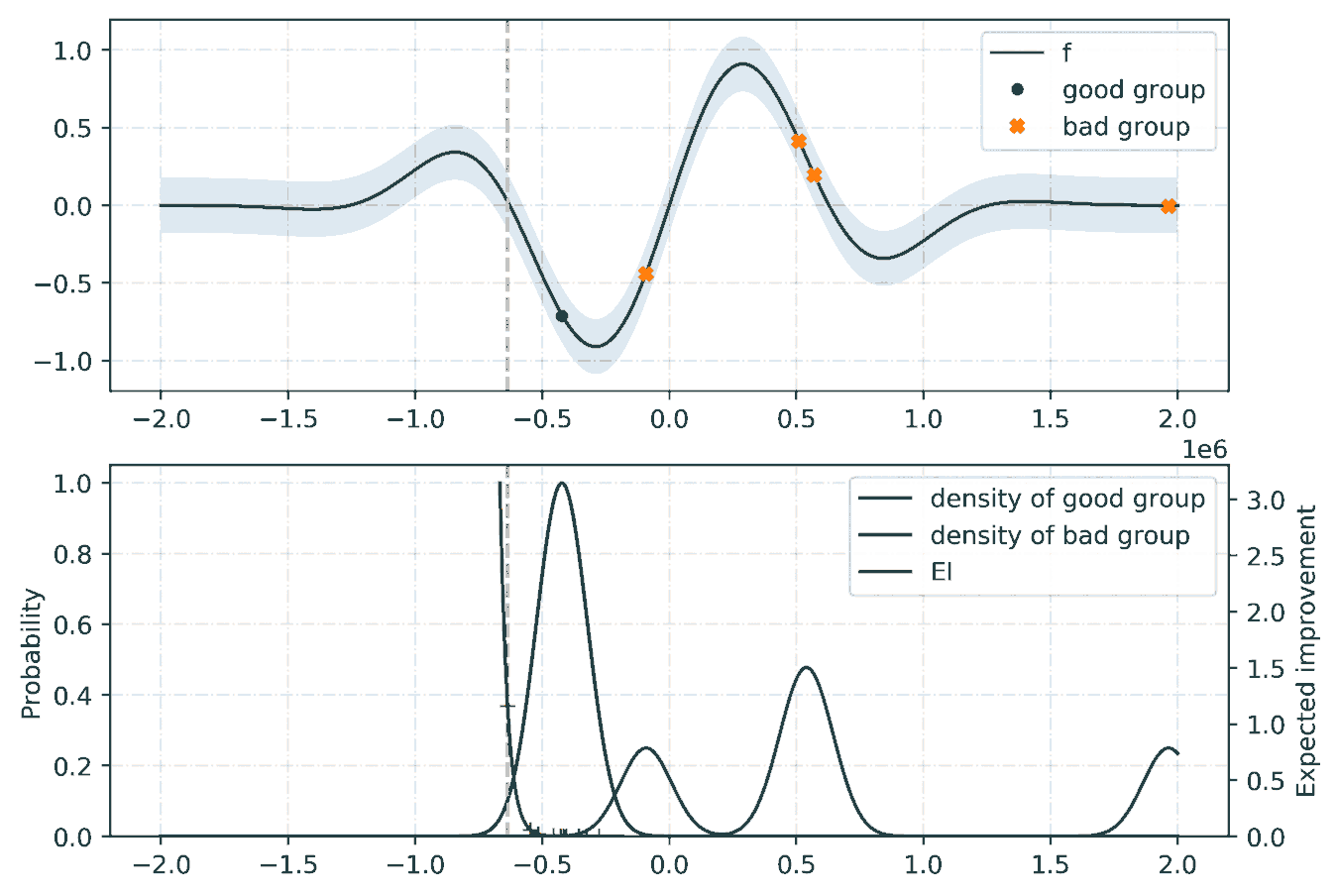
For the tunning of the hyper-parameters, we rely on a python library called hyperopt with the Tree-structured Parzen Estimator (TPE) [2] as the optimization algorithm. Given a set of hyper-parameters \(x\) with an associated quality score \(y\), the idea of TPE is to compute a tree of Parzen estimators \(P (x | y)\) and \(P(y)\). To initialize the algorithm, the TPE starts from a random search. Then, it splits the results into two groups: the best performing ones and the reset by defining a splitting value \(\tilde{y}\). The likelihood probability for being in each of the groups is modeled as:
where the two densities \(\mathcal{L}\) and \(\mathcal{G}\) are modeled using kernel density estimators which are a simple average of the kernels centered on existing data points. \(P(y)\) is modeled using the fact that \(P(y < \tilde{y}) = 0.75\) if \(\mathcal{G}\) models the upper quartile. Finally, the next set of hyper-parameters are taken as the maximizer of \(\mathcal{L}(x) / \mathcal{G}(x)\) [3] as shown below: